Data Analysis Showdown: Comparing SQL, Python, and esProc SPL

Talk is cheap; let’s show the codes.

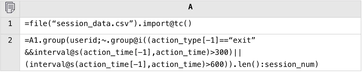
1. User Session Count

User behavior data table

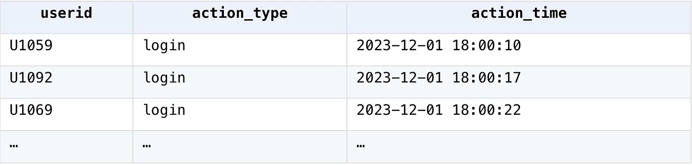
A session is considered over if a user does not take any action within 10 minutes, or if they do not log in within 5 minutes after logging out. Calculate the number of sessions for each user.

SPL

SQL

WITH login_data AS (
    SELECT userid, action_type, action_time,
        LAG(action_time) OVER (PARTITION BY userid ORDER BY action_time) AS prev_time,
        LAG(action_type) OVER (PARTITION BY userid ORDER BY action_time) AS prev_action
    FROM session_data)
SELECT userid, COUNT(*) AS session_count
FROM (
    SELECT userid, action_type, action_time, prev_time, prev_action,
        CASE
            WHEN prev_time IS NULL OR (action_time - prev_time) > 60 
                OR (prev_action = 'exit' AND (action_time - prev_time) > 300 )
            THEN 1
            ELSE 0
        END AS is_new_session
    FROM login_data)
WHERE is_new_session = 1
GROUP BY userid;

Python

login_data = pd.read_csv("session_data.csv")
login_data['action_time'] = pd.to_datetime(login_data['action_time'])
grouped = login_data.groupby("userid")
session_count = {}
for uid, sub_df in grouped:
    session_count[uid] = 0
    start_index = 0
    for i in range(1, len(sub_df)):
        current = sub_df.iloc[i]
        last = sub_df.iloc[start_index]
        last_action = last['action_type']
        if (current["action_time"] - last["action_time"]).seconds > 600 or \
            (last_action=="exit" and (current["action_time"] - last["action_time"]).seconds > 300):
            session_count[uid] += 1
        start_index = i
    session_count[uid] += 1
session_cnt = pd.DataFrame(list(session_count.items()), columns=['UID', 'session_count'])

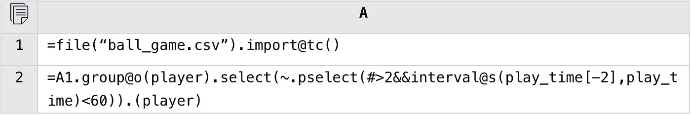
2. Count the players who score 3 times in a row within 1 minute

Score table of a ball game

SPL

SQL

WITH numbered_scores AS (
    SELECT team, player, play_time, score,
        ROW_NUMBER() OVER (ORDER BY play_time) AS rn
    FROM ball_game)
SELECT DISTINCT s1.player
FROM numbered_scores s1
    JOIN numbered_scores s2 ON s1.player = s2.player AND s1.rn = s2.rn - 1
    JOIN numbered_scores s3 ON s1.player = s3.player AND s1.rn = s3.rn - 2
WHERE (s3.play_time - s1.play_time) <60 ;

Python

df = pd.read_csv("ball_game.csv")
df["play_time"] = pd.to_datetime(df["play_time"])
result_players = []
player = None
start_index = 0
consecutive_scores = 0
for i in range(len(df)-2):
    current = df.iloc[i]
    if player != current["player"]:
        player = current["player"]
        consecutive_scores = 1
    else:
        consecutive_scores += 1
    last2 = df.iloc[i-2] if i >=2 else None
    if consecutive_scores >= 3 and (current['play_time'] - last2['play_time']).seconds < 60:
        result_players.append(player)
result_players = list(set(result_players))

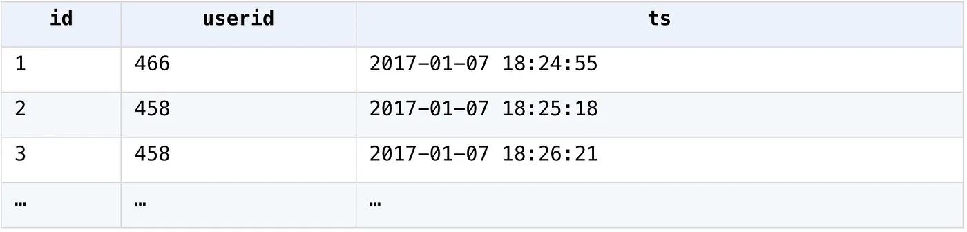
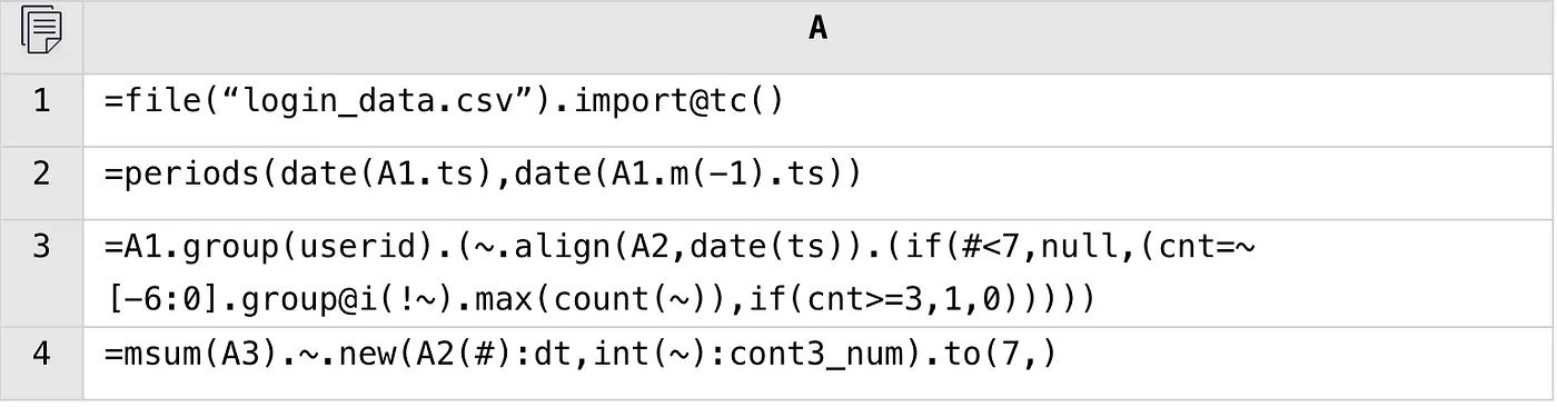
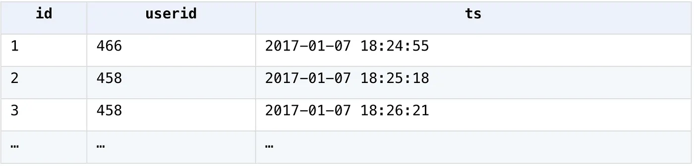
3. Calculate the number of users who are active for three consecutive days within every 7 days

User login data table

SPL

SQL

WITH all_dates AS (
    SELECT DISTINCT TRUNC(ts) AS login_date
    FROM login_data),
user_login_counts AS (
    SELECT userid, TRUNC(ts) AS login_date, 
        (CASE WHEN COUNT(*)>=1 THEN 1 ELSE 0 END) AS login_count
    FROM login_data
    GROUP BY userid, TRUNC(ts)),
whether_login AS (
    SELECT u.userid, ad.login_date, NVL(ulc.login_count, 0) AS login_count
    FROM all_dates ad
    CROSS JOIN (
        SELECT DISTINCT userid
        FROM login_data) u
    LEFT JOIN user_login_counts ulc
    ON u.userid = ulc.userid
    AND ad.login_date = ulc.login_date
    ORDER BY u.userid, ad.login_date),
whether_login_rn AS (
    SELECT userid,login_date,login_count,ROWNUM AS rn 
    FROM whether_login),
whether_eq AS(
    SELECT userid,login_date,login_count,rn,
        (CASE 
            WHEN LAG(login_count,1) OVER (ORDER BY rn)= login_count 
                AND login_count =1 AND LAG(userid,1) OVER (ORDER BY rn)=userid 
            THEN 0 
            ELSE 1 
        END) AS wether_e 
    FROM whether_login_rn
),
numbered_sequence AS (
    SELECT userid,login_date,login_count,rn, wether_e,
        SUM(wether_e) OVER (ORDER BY rn) AS lab
    FROM whether_eq),
consecutive_logins_num AS (
    SELECT userid,login_date,login_count,rn, wether_e,lab,
        (SELECT (CASE WHEN max(COUNT(*))<3 THEN 0 ELSE 1 END)
        FROM numbered_sequence b
        WHERE b.rn BETWEEN a.rn - 6 AND a.rn
        AND b.userid=a.userid
        GROUP BY b. lab) AS cnt
    FROM numbered_sequence a)
SELECT login_date,SUM(cnt) AS cont3_num
FROM consecutive_logins_num
WHERE login_date>=(SELECT MIN(login_date) FROM all_dates)+6
GROUP BY login_date
ORDER BY login_date;

Python

df = pd.read_csv("login_data.csv")
df["ts"] = pd.to_datetime(df["ts"]).dt.date
grouped = df.groupby("userid")
aligned_dates = pd.date_range(start=df["ts"].min(), end=df["ts"].max(), freq='D')
user_date_wether_con3days = []
for uid, group in grouped:
    group = group.drop_duplicates('ts')
    aligned_group = group.set_index("ts").reindex(aligned_dates)
    consecutive_logins = aligned_group.rolling(window=7)
    n = 0
    date_wether_con3days = []
    for r in consecutive_logins:
        n += 1
        if n<7:
            continue
        else:
            ds = r['userid'].isna().cumsum()
            cont_login_times = r.groupby(ds).userid.count().max()
            wether_cont3days = 1 if cont_login_times>=3 else 0
            date_wether_con3days.append(wether_cont3days)
    user_date_wether_con3days.append(date_wether_con3days)
arr = np.array(user_date_wether_con3days)
day7_cont3num = np.sum(arr,axis=0)
result = pd.DataFrame({'dt':aligned_dates[6:],'cont3_num':day7_cont3num})

4. Calculate the next-day retention rate of new users per day

User login data table

SPL

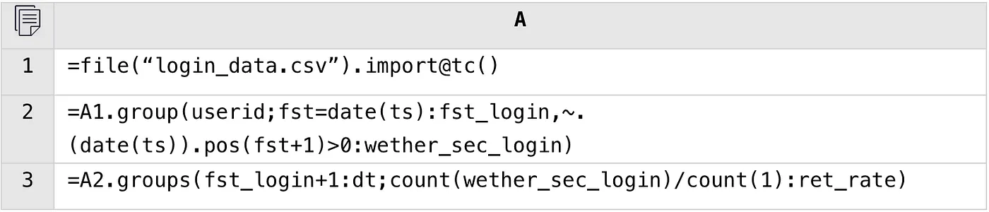
A2: Group by user; record the first login date and check whether the user logs in the next day.

A3: Calculate the next-day retention rate based on the login date of the next day.

SQL

WITH first_login AS (
    SELECT userid, MIN(TRUNC(ts)) AS first_login_date
    FROM login_data
    GROUP BY userid),
next_day_login AS (
    SELECT DISTINCT(fl.userid), fl.first_login_date, TRUNC(ld.ts) AS next_day_login_date
    FROM first_login fl
    LEFT JOIN login_data ld ON fl.userid = ld.userid
    WHERE TRUNC(ld.ts) = fl.first_login_date + 1),
day_new_users AS(
    SELECT first_login_date,COUNT(*) AS new_user_num
    FROM first_login
    GROUP BY first_login_date),
next_new_users AS(
    SELECT next_day_login_date, COUNT(*) AS next_user_num
    FROM next_day_login
    GROUP BY next_day_login_date),
all_date AS(
    SELECT DISTINCT(TRUNC(ts)) AS login_date
    FROM login_data)
SELECT all_date.login_date+1 AS dt,dn. new_user_num,nn. next_user_num,
    (CASE 
        WHEN nn. next_day_login_date IS NULL 
        THEN 0 
        ELSE nn.next_user_num 
    END)/dn.new_user_num AS ret_rate
FROM all_date
    JOIN day_new_users dn ON all_date.login_date=dn.first_login_date
    LEFT JOIN next_new_users nn ON dn.first_login_date+1=nn. next_day_login_date
ORDER BY all_date.login_date;

Python

df = pd.read_csv("login_data.csv")
df["ts"] = pd.to_datetime(df["ts"]).dt.date
gp = df.groupby('userid')
row = []
for uid,g in gp:
    fst_dt = g.iloc[0].ts
    sec_dt = fst_dt + pd.Timedelta(days=1)
    all_dt = g.ts.values
    wether_sec_login = sec_dt in all_dt
    row.append([uid,fst_dt,sec_dt,wether_sec_login])
user_wether_ret_df = pd.DataFrame(row,columns=['userid','fst_dt','sec_dt','wether_sec_login'])
result = user_wether_ret_df.groupby('sec_dt').apply(lambda x:x['wether_sec_login'].sum()/len(x))

5. Calculate the increase of stock price on the day when it is higher than those on the previous and next 5 days

Stock price data table

SPL

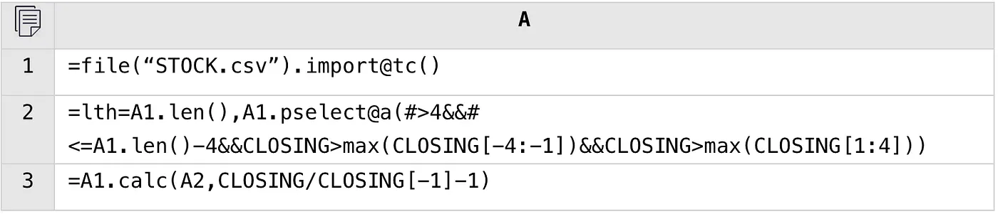
A2: The position where the stock price is higher than those of the previous and next 5 days.
A3: Calculate the increase at that time.

SQL

SELECT closing/closing_pre-1 AS raise
FROM(
    SELECT dt, closing, ROWNUM AS rn,
        MAX(closing) OVER (
            ORDER BY dt ROWS BETWEEN 5 PRECEDING AND 1 PRECEDING) AS max_pre,
        MAX(closing) OVER (
            ORDER BY dt ROWS BETWEEN 1 FOLLOWING AND 5 FOLLOWING) AS max_suf,
        LAG(closing,1) OVER (ORDER BY dt) AS closing_pre
    FROM stock)
WHERE rn>5 AND rn<=(select count(*) FROM stock)-5
    AND CLOSING>max_pre AND CLOSING>max_suf;

Python

stock_price_df = pd.read_csv('STOCK.csv')
price_increase_list = []
for i in range(5, len(stock_price_df)-5):
    if stock_price_df['CLOSING'][i] > max(stock_price_df['CLOSING'][i-5:i]) and \
    stock_price_df['CLOSING'][i] > max(stock_price_df['CLOSING'][i+1:i+6]):
        price_increase = stock_price_df['CLOSING'][i] / stock_price_df['CLOSING'][i-1]-1
        price_increase_list.append(price_increase)
result = price_increase_list

esProc SPL is open-source and here's the Open-Source Address.